
Improving CLIP’s Image Recognition: A Guide to Targeted Fine-Tuning
Step-by-step methods to align pre-trained vision features with your data


Here is a tutorial on fine tuning CLIP image encoder for image classification task. The goal of this project is to develop an image classification system capable of categorising images based on their visual content.
The training data consists of labeled images, organized in a class-wise directory structure where each folder represents a distinct category and contains multiple corresponding examples. Structure the /data directory as follows,
# /data
.
├── cat
│   ├── 0.jpg
│   ├── 1.jpg
│   ├── 2.jpg
│   └── 3.jpg
└── dog
    ├── 0.jpg
    ├── 1.jpg
    ├── 2.jpg
    └── 3.jpg
Methodology ☀️
To tackle this image classification, we can leverage contrastive learning.
Contrastive learning is a technique where a model learns to distinguish if images are similar. Images of the same class are coined as positive pairs, while images of different classes are negative pairs.
In contrastive learning, the model contrasts positive and negative pairs, where similar images are pulled closer together and dissimilar images are pushed further apart from one another in the embedding space. The embedding space is a learned representation space where images are mapped to vectors.
The contrastive loss function, such as the InfoNCE loss, aims to minimize the distance between positive pairs and maximize the distance between negative pairs. It is particularly effective in self-supervised learning without labels.
Data Preprocessing
For machine to "see" the images, they must first be converted into numerical representations called embeddings. We will initially represent each image as a simple 2-dimensional vector. However, in practice, models like CLIP generate high-dimensional embeddings e.g., 512 dimensions that capture richer information.
After converting the images and normalizing the resulting embedding vectors, the data looks like this:
| Class | Image   | Raw Embedding (x, y) | Normalized Embedding (x, y) |
| cat   | 0.jpg   | [1.2, 0.9]           | [0.800, 0.600]              |
Subsequently, a scaling hyperparameter called temperature is often applied to this similarity matrix, typically by dividing the matrix elements by it.
For images cat/0.jpg, cat/1.jpg, dog/0.jpg, dog/1.jpg, the corresponding labels would be:
labels = torch.tensor([ 0, 0, 1, 1])where class 0 is cat and class 1 is dog.
The temperature hyperparameter (τ) adjusts the model's sensitivity to the similarity scores. By scaling the similarity scores, it modifies how strongly the model differentiates between pairs of embeddings based on their similarity.
When a smaller value of τ ( nearer to 0 ) is used, the loss function is more sensitive to small differences in similarity scores. The exponential of the dot product exaggerates these differences, leading to a sharper probability distribution in the denominator of the logarithmic term.
As a result, the model penalised stronger for even slightly incorrect similarities. In another words, it focuses more on fine-grained distinctions of the training data.
Lower Temperature:
Sharper similarity distribution: The model becomes more confident about its assignments based on similarity scores
Amplifies differences between similarity scores: Small differences in high similarity scores lead to larger differences in the resulting probabilities (after softmax)
Increases penalty for hard negatives: The model focuses more strongly on separating embeddings that are not in the same class but have relatively high similarity
Higher temperature "melts" the probability distribution, where samples are more evenly spread out in the embedding space
Deciding Factor:
Low temperature: Use when you want the model to learn strong separation between classes and create tightly clustered embeddings for items within the same class. Emphasizes discriminating between positives and hard negatives. Can sometimes lead to instability if too low.
High temperature: Use when you want a softer probability distribution. This treats negative pairs more uniformly, potentially preventing the model from focusing too narrowly on only the hardest negatives early in training. It allows for smoother gradients from a wider range of pairs.
Looking back at the similarity scores derived from our 2D example embeddings, we observe high cosine similarity values for embeddings within the same class (cat-cat, dog-dog), and lower scores for cross-class pairs (cat-dog). This indicates a good initial separation between the classes in the embedding space, even before fine-tuning.
The diagonal elements of the computed similarity matrix correspond to the similarity of each embedding with itself.
Since the embeddings are normalized, these values should theoretically be exactly 1.0 (cosine_similarity(v, v) = 1 for ||v||=1). In practice, due to standard floating-point arithmetic precision limits in computations, the calculated diagonal values might be extremely close but not precisely 1.0.
The Loss Formula 🌾
Here we are using supervised contrastive (SupCon) loss,
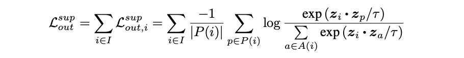
The numerator:
Focuses only on the similarity between anchor `i` and one specific positive
Measures the similarity between the anchor sample (z_i) and one specific positive sample (z_p) that belongs to the same class.
The denominator:
Considers the anchor `i` and all other samples `a` in the batch
Represents the sum of similarities between the anchor (z_i) and all other samples (z_a) in the batch (both positives and negatives).
The fraction
Like a softmax function, it calculates a normalised score (probability like value) representing how well the positive sample `p` is the correct match for anchor sample `i`, given the similarities of `i` to all available candidates `a`.
The loss function encourages the model to make this fraction to approach 1 for every positive `p`
Thinking further about the loss.. 💭
That means, similar images should have a higher numerator where the cosine similarity should be closer to 1. The fraction therefore is larger for positive pair and together with - log, the loss becomes a smaller value closer to 0.
However, if the scaled similarities are large positive numbers, exponentiating these large numbers potentially exceed the limits of standard floating point numbers resulting in numerical overflow and breaking the calculation.
Therefore, we can apply a constant shift to this softmax-like calculation to obtain a more stable version before the exponentiation.
logits_max, _ = torch.max(similarity_matrix, dim=1, keepdim=True)
logits = similarity_matrix - logits_max.detach()
As a result, the largest value in each row of the logits should be 0 and all other values should be less than or equal to 0.
Mask Generation 🎭
To correctly calculate the Supervised Contrastive loss components using matrix operations on the full `logits` matrix, we typically need two masks based on item indices and labels within the batch:
Self-Mask (Exclusion Mask for Denominator):
The denominator requires excluding the anchor's similarity with itself (`k=i`). We create a self_mask that is 1 everywhere except for the diagonal, which is 0.
batch_size = features.shape[0] # Or logits.shape[0]
device = features.device # Or logits.device

# Creates a mask with 0 on diagonal, 1 elsewhere
self_mask = torch.ones_like(logits, device=device)
self_mask.fill_diagonal_(0)

# Alternative using scatter:
self_mask = torch.scatter(
    torch.ones_like(logits, device=device),
    1,
    torch.arange(batch_size, device=device).view(-1, 1),
    0
 ).to(device)

# --  SELF MASK OUTPUT --
tensor([[0., 1., 1., 1.],
        [1., 0., 1., 1.],
        [1., 1., 0., 1.],
        [1., 1., 1., 0.]])
Positive Pair Mask (Label Mask for Loss Calculation):
To calculate the final loss, we need to identify all `(i, p)` pairs in the batch that belong to the same class. This mask is generated by comparing labels. It is 1 where `label[i] == label[k]` and 0 otherwise.
It must also incorporate the self-mask logic to ensure `i≠k`. So, `positive_mask[i, k] = 1` if and only if `label[i] == label[k]` AND `i ≠ k`. This mask selects the terms corresponding to positive pairs `p` needed for the inner summation `Σ_{p ∈ P(i)}` and helps calculate the number of positives `|P(i)|`
We leverage the labels tensor for this.
# Assumes 'labels' is a 1D tensor of size [batch_size]
labels_reshaped = labels.contiguous().view(-1, 1)

# Create mask where True if labels match (broadcasting [B,1] vs [1,B])
positive_mask = torch.eq(labels_reshaped, labels_reshaped.T).float().to(device)

# Exclude self-comparisons (diagonal) from being positive pairs
positive_mask = mask * self_mask

# -- OUTPUT OF POSITIVE MASK --
tensor([[1., 1., 0., 0.],
        [1., 1., 0., 0.],
        [0., 0., 1., 1.],
        [0., 0., 1., 1.]])

# alternatively, positive mask can be created with:
positive_mask = (labels.unsqueeze(0) == labels.unsqueeze(1)).float()

# Exclude self-comparisons (diagonal) from being positive pairs
positive_mask.fill_diagonal_(0)

# -- FINAL POSITIVE MASK EXCLUDING SELF --
tensor([[0., 1., 0., 0.],
        [1., 0., 0., 0.],
        [0., 0., 0., 1.],
        [0., 0., 1., 0.]])
Continuing from the mask generation, let's see how the self_mask is used to calculate the denominator term defined earlier.
Recall that the self_mask is designed to ignore the self-similarity term (k=i). We can apply this mask after exponentiating the entire logits matrix. Multiplying the exponentiated logits by the self_mask effectively zeros out the diagonal (i=k) terms. Summing the result across the k dimension then yields the correct denominator sum for each anchor `i`, as we need to exclude self-similarity term (k=i) from the sum.
# Calculate exp(logits[i, k]) for all k != i
# Note: 'logits' are the scaled and stabilized similarities
exp_logits_all_non_self = torch.exp(logits) * self_mask

# Calculate Denominator: Sum over k where k != i for each anchor i
sum_exp_logits_all_non_self = exp_logits_all_non_self.sum(dim=1, keepdim=True)
Log Probability Calculation
Instead of calculating the fraction (Numerator / Denominator) and then taking -log, the code uses the more stable `log_prob = logits - log(denominator)`.
This reduces the risk of intermediate overflow/underflow during the sum and log steps compared to doing it naively.
log_prob = logits - torch.log(sum_exp_logits_all_non_self + 1e-12)
Loss Calculation
Finally we are ready to put things in the loss function, we will be using the `positive mask` which identifies the positive pairs to calculate the loss.
The loss is the average loss contribution across all positive and all anchors in the batch.
# positive_mask * log_prob zeros out log_prob values for all non-positive pairs
# (negatives and self-pairs), keeping only log_prob[i, p] where p is a positive for i

# positive_mask.sum(1) calculates |P(i)|

mean_log_prob_positive = (positive_mask * log_prob).sum(1) / (positive_mask.sum(1).clamp(min=1e-12))

# Final loss is the mean over all anchors
loss = -mean_log_prob_positive.mean()
Time to Finetune 🔆
The image encoder in CLIP follows the vision transformer architecture (ViT). The transformer encoder core consists of stacked transformer blocks which are multiple identical layers stacked sequentially.
After passing through the transformer blocks, the output state corresponding to the initial `[class]` token position is used as the aggregated representation of the image. The vector then undergoes these final processing layers:
Final layer normalisation `ln_post`:
This is a `nn.LayerNorm` that helps with stablising the vector representation's statistics e.g mean, variance
Projection layer `proj`:
This is a `nn.Linear` that maps normalised features from `ln_post` into the target joint embedding space. The weights of `proj` are optimised during pre-training to align image embeddings with the corresponding text embeddings under a contrastive loss.
In our scenario, our task is repurposed to image classification defined by supervised contrastive loss, operating on existing class label. As such, introducing a new MLP projector is suitable and the loss is calculated on the output of this new projector.
While the original image-text mapping objective is discarded, `visual_model.proj` still serves as the final learned transformation applied by the pre-trained network components before the features reach our task-specific `self.projector`.
By unfreezing `proj`, we allow gradients originating from the SupCon loss (calculated further down the network) to flow back and update proj's weights. This enables the layer to adapt its mapping, refining the features it outputs to be more discriminative or better suited for the class-based contrastive task, thereby providing a higher quality input to `self.projector`.
Optimizer Configuration
We will be using `AdamW` as the optimizer algorithm, initialising it to handle only the parameters marked as trainable and setting the learning rate.
# Filter parameters that require gradients
# Use model.parameters() to include both encoder (if parts are unfrozen) and projector
params_to_train = filter(lambda p: p.requires_grad, model.parameters())

# Instantiate the optimizer
optimizer = torch.optim.AdamW(params_to_train, lr=lr, weight_decay=weight_decay)
Dataset & Dataloader
A custom PyTorch Dataset is required to load images and their integer class labels.
Loss Function
Instantiate the Supervised Contrastive loss function with the desired temperature hyperparameter. Use `torch.utils.data.DataLoader` to create batches, ensuring a sufficiently large batch_size and `setting shuffle=True` for training.
loss = supervised_contrastive_loss(embeddings, labels, temperature)With the optimizer, data pipeline, and loss function ready, the next step is the core training process.
for epoch in range(num_epochs):
        model.train() # set model to training mode
        total_train_loss = 0.0
        batches_processed = 0

        for batch_idx, (images, labels) in enumerate(trainloader):
                optmizer.zero_grad() # reset optimizer gradient
                images, labels = images.to(device), labels.to(device)
                current_batch_size = labels.shape[0]

                embeddings = visual_model(images)
                loss = contrastive_loss(embeddings, labels, temperature)

                # --- Handle potential NaN/Inf loss ---
                if torch.isnan(loss) or torch.isinf(loss):
                        logger.warning(f"Epoch {epoch+1}, Batch {batch_idx+1}: NaN or Inf loss! Skipping.")
                        continue

                # Backforward pass
                loss.backward()

                # Update the trainable model weights based on the computed gradients
                optimizer.step()

                loss_item = loss.item()
                total_train_loss += loss_item
                batches_processed += 1

                if batches_processed > 0:
                        avg_epoch_loss = total_train_loss / batches_processed
                        logger.info(f"Epoch [{epoch+1}/{num_epochs}] Average Training Loss: {avg_epoch_loss:.4f}")
                else:
                        logger.warning(f"Epoch [{epoch+1}/{num_epochs}]: No batches processed successfully.")
Evaluation Metrics
Once the CLIP image encoder has been fine-tuned using contrastive learning, we need methods to assess the quality of the resulting image embeddings, especially since the model typically lacks a classification head trained during this phase. Standard classification accuracy isn't directly available. Instead, we evaluate the characteristics of the learned embedding space using proxy tasks like k-Nearest Neighbors (k-NN) classification, often supplemented by visualization.
k-NN Classification
This metric evaluates the local structure and clustering quality of the embedding space. The underlying principle is that embeddings of images from the same class should reside closer to each other than embeddings from different classes after fine-tuning.
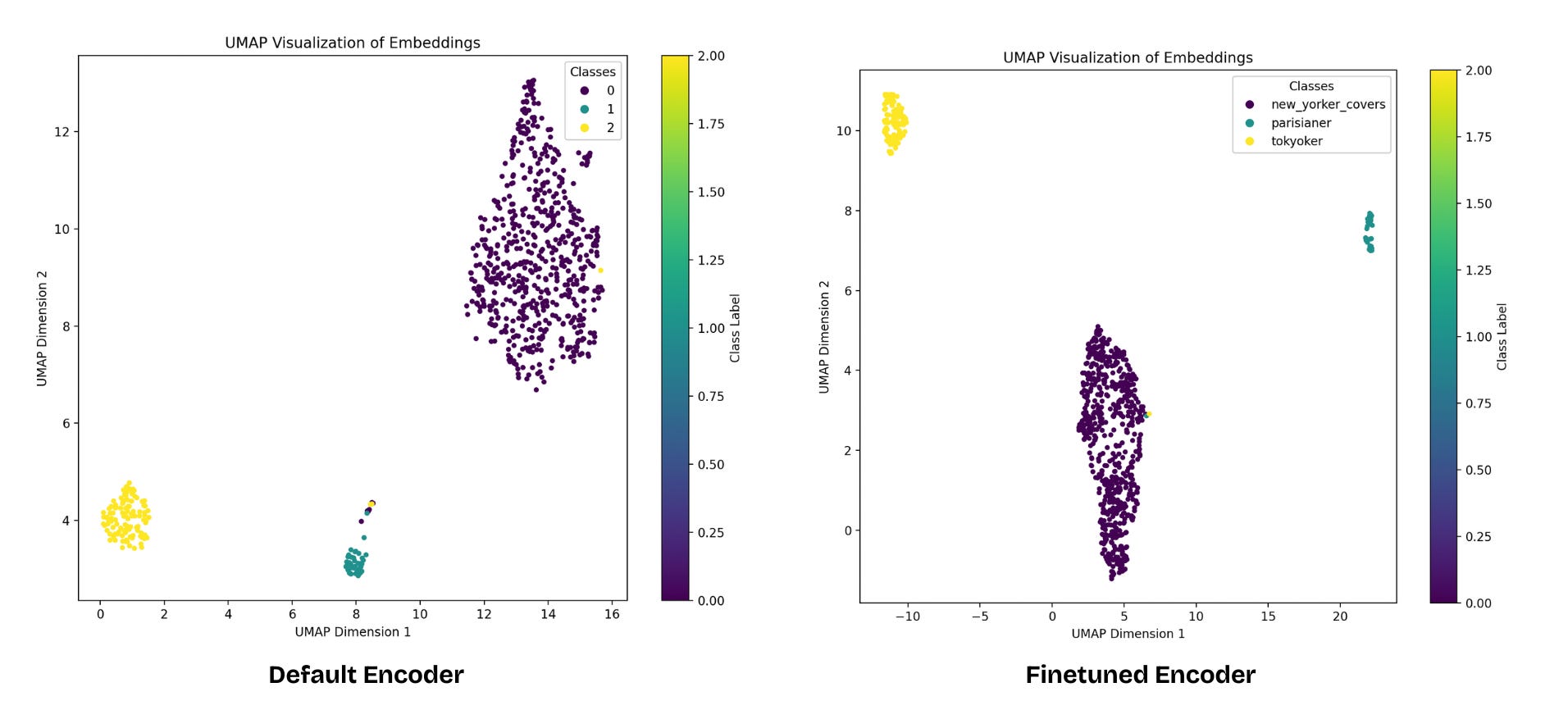
Embedding Visualisation
Visual inspection provides qualitative insights into the structure of the embedding space and the effectiveness of the fine-tuning process. From the visualisation, we observe that the embeddings of the same class cluster tighter together with the finetuned image encoder.
Conclusion
Fine tuning the CLIP image encoder allows for the adaption of embeddings to better capture the specific visual relationships within a target domain. This helps to improve the quality of embedding space customised to a specific task in various downstream applications. Consider experimenting further with different hyper parameters, datasets to observe how these embeddings behave. Keep coding!